$$ \newcommand{\bone}{\mathbf{1}} \newcommand{\bbeta}{\mathbf{\beta}} \newcommand{\bdelta}{\mathbf{\delta}} \newcommand{\bepsilon}{\mathbf{\epsilon}} \newcommand{\blambda}{\mathbf{\lambda}} \newcommand{\bomega}{\mathbf{\omega}} \newcommand{\bpi}{\mathbf{\pi}} \newcommand{\bphi}{\mathbf{\phi}} \newcommand{\bvphi}{\mathbf{\varphi}} \newcommand{\bpsi}{\mathbf{\psi}} \newcommand{\bsigma}{\mathbf{\sigma}} \newcommand{\btheta}{\mathbf{\theta}} \newcommand{\btau}{\mathbf{\tau}} \newcommand{\ba}{\mathbf{a}} \newcommand{\bb}{\mathbf{b}} \newcommand{\bc}{\mathbf{c}} \newcommand{\bd}{\mathbf{d}} \newcommand{\be}{\mathbf{e}} \newcommand{\boldf}{\mathbf{f}} \newcommand{\bg}{\mathbf{g}} \newcommand{\bh}{\mathbf{h}} \newcommand{\bi}{\mathbf{i}} \newcommand{\bj}{\mathbf{j}} \newcommand{\bk}{\mathbf{k}} \newcommand{\bell}{\mathbf{\ell}} \newcommand{\bm}{\mathbf{m}} \newcommand{\bn}{\mathbf{n}} \newcommand{\bo}{\mathbf{o}} \newcommand{\bp}{\mathbf{p}} \newcommand{\bq}{\mathbf{q}} \newcommand{\br}{\mathbf{r}} \newcommand{\bs}{\mathbf{s}} \newcommand{\bt}{\mathbf{t}} \newcommand{\bu}{\mathbf{u}} \newcommand{\bv}{\mathbf{v}} \newcommand{\bw}{\mathbf{w}} \newcommand{\bx}{\mathbf{x}} \newcommand{\by}{\mathbf{y}} \newcommand{\bz}{\mathbf{z}} \newcommand{\bA}{\mathbf{A}} \newcommand{\bB}{\mathbf{B}} \newcommand{\bC}{\mathbf{C}} \newcommand{\bD}{\mathbf{D}} \newcommand{\bE}{\mathbf{E}} \newcommand{\bF}{\mathbf{F}} \newcommand{\bG}{\mathbf{G}} \newcommand{\bH}{\mathbf{H}} \newcommand{\bI}{\mathbf{I}} \newcommand{\bJ}{\mathbf{J}} \newcommand{\bK}{\mathbf{K}} \newcommand{\bL}{\mathbf{L}} \newcommand{\bM}{\mathbf{M}} \newcommand{\bN}{\mathbf{N}} \newcommand{\bP}{\mathbf{P}} \newcommand{\bQ}{\mathbf{Q}} \newcommand{\bR}{\mathbf{R}} \newcommand{\bS}{\mathbf{S}} \newcommand{\bT}{\mathbf{T}} \newcommand{\bU}{\mathbf{U}} \newcommand{\bV}{\mathbf{V}} \newcommand{\bW}{\mathbf{W}} \newcommand{\bX}{\mathbf{X}} \newcommand{\bY}{\mathbf{Y}} \newcommand{\bZ}{\mathbf{Z}} \newcommand{\calA}{\mathcal{A}} \newcommand{\calB}{\mathcal{B}} \newcommand{\calC}{\mathcal{C}} \newcommand{\calD}{\mathcal{D}} \newcommand{\calE}{\mathcal{E}} \newcommand{\calF}{\mathcal{F}} \newcommand{\calG}{\mathcal{G}} \newcommand{\calH}{\mathcal{H}} \newcommand{\calI}{\mathcal{I}} \newcommand{\calJ}{\mathcal{J}} \newcommand{\calK}{\mathcal{K}} \newcommand{\calL}{\mathcal{L}} \newcommand{\calM}{\mathcal{M}} \newcommand{\calN}{\mathcal{N}} \newcommand{\calO}{\mathcal{O}} \newcommand{\calP}{\mathcal{P}} \newcommand{\calQ}{\mathcal{Q}} \newcommand{\calR}{\mathcal{R}} \newcommand{\calS}{\mathcal{S}} \newcommand{\calT}{\mathcal{T}} \newcommand{\calU}{\mathcal{U}} \newcommand{\calV}{\mathcal{V}} \newcommand{\calW}{\mathcal{W}} \newcommand{\calX}{\mathcal{X}} \newcommand{\calY}{\mathcal{Y}} \newcommand{\calZ}{\mathcal{Z}} \newcommand{\R}{\mathbb{R}} \newcommand{\C}{\mathbb{C}} \newcommand{\N}{\mathbb{N}} \newcommand{\Z}{\mathbb{Z}} \newcommand{\F}{\mathbb{F}} \newcommand{\Q}{\mathbb{Q}} \DeclareMathOperator*{\argmax}{arg\,max} \DeclareMathOperator*{\argmin}{arg\,min} \newcommand{\nnz}[1]{\mbox{nnz}(#1)} \newcommand{\dotprod}[2]{\langle #1, #2 \rangle} \newcommand{\ignore}[1]{} \let\Pr\relax \DeclareMathOperator*{\Pr}{\mathbf{Pr}} \newcommand{\E}{\mathbb{E}} \DeclareMathOperator*{\Ex}{\mathbf{E}} \DeclareMathOperator*{\Var}{\mathbf{Var}} \DeclareMathOperator*{\Cov}{\mathbf{Cov}} \DeclareMathOperator*{\stddev}{\mathbf{stddev}} \DeclareMathOperator*{\avg}{avg} \DeclareMathOperator{\poly}{poly} \DeclareMathOperator{\polylog}{polylog} \DeclareMathOperator{\size}{size} \DeclareMathOperator{\sgn}{sgn} \DeclareMathOperator{\dist}{dist} \DeclareMathOperator{\vol}{vol} \DeclareMathOperator{\spn}{span} \DeclareMathOperator{\supp}{supp} \DeclareMathOperator{\tr}{tr} \DeclareMathOperator{\Tr}{Tr} \DeclareMathOperator{\codim}{codim} \DeclareMathOperator{\diag}{diag} \newcommand{\PTIME}{\mathsf{P}} \newcommand{\LOGSPACE}{\mathsf{L}} \newcommand{\ZPP}{\mathsf{ZPP}} \newcommand{\RP}{\mathsf{RP}} \newcommand{\BPP}{\mathsf{BPP}} \newcommand{\P}{\mathsf{P}} \newcommand{\NP}{\mathsf{NP}} \newcommand{\TC}{\mathsf{TC}} \newcommand{\AC}{\mathsf{AC}} \newcommand{\SC}{\mathsf{SC}} \newcommand{\SZK}{\mathsf{SZK}} \newcommand{\AM}{\mathsf{AM}} \newcommand{\IP}{\mathsf{IP}} \newcommand{\PSPACE}{\mathsf{PSPACE}} \newcommand{\EXP}{\mathsf{EXP}} \newcommand{\MIP}{\mathsf{MIP}} \newcommand{\NEXP}{\mathsf{NEXP}} \newcommand{\BQP}{\mathsf{BQP}} \newcommand{\distP}{\mathsf{dist\textbf{P}}} \newcommand{\distNP}{\mathsf{dist\textbf{NP}}} \newcommand{\eps}{\epsilon} \newcommand{\lam}{\lambda} \newcommand{\dleta}{\delta} \newcommand{\simga}{\sigma} \newcommand{\vphi}{\varphi} \newcommand{\la}{\langle} \newcommand{\ra}{\rangle} \newcommand{\wt}[1]{\widetilde{#1}} \newcommand{\wh}[1]{\widehat{#1}} \newcommand{\ol}[1]{\overline{#1}} \newcommand{\ul}[1]{\underline{#1}} \newcommand{\ot}{\otimes} \newcommand{\zo}{\{0,1\}} \newcommand{\co}{:} %\newcommand{\co}{\colon} \newcommand{\bdry}{\partial} \newcommand{\grad}{\nabla} \newcommand{\transp}{^\intercal} \newcommand{\inv}{^{-1}} \newcommand{\symmdiff}{\triangle} \newcommand{\symdiff}{\symmdiff} \newcommand{\half}{\tfrac{1}{2}} \newcommand{\bbone}{\mathbbm 1} \newcommand{\Id}{\bbone} \newcommand{\SAT}{\mathsf{SAT}} \newcommand{\bcalG}{\boldsymbol{\calG}} \newcommand{\calbG}{\bcalG} \newcommand{\bcalX}{\boldsymbol{\calX}} \newcommand{\calbX}{\bcalX} \newcommand{\bcalY}{\boldsymbol{\calY}} \newcommand{\calbY}{\bcalY} \newcommand{\bcalZ}{\boldsymbol{\calZ}} \newcommand{\calbZ}{\bcalZ} $$

2022

  1. Rinon Gal, Yuval Alaluf, Yuval Atzmon, and 4 more authors
    Aug 2022

    Paper Abstract

    Text-to-image models offer unprecedented freedom to guide creation through natural language. Yet, it is unclear how such freedom can be exercised to generate images of specific unique concepts, modify their appearance, or compose them in new roles and novel scenes. In other words, we ask: how can we use language-guided models to turn our cat into a painting, or imagine a new product based on our favorite toy? Here we present a simple approach that allows such creative freedom. Using only 3-5 images of a user-provided concept, like an object or a style, we learn to represent it through new "words" in the embedding space of a frozen text-to-image model. These "words" can be composed into natural language sentences, guiding personalized creation in an intuitive way. Notably, we find evidence that a single word embedding is sufficient for capturing unique and varied concepts. We compare our approach to a wide range of baselines, and demonstrate that it can more faithfully portray the concepts across a range of applications and tasks. Our code, data and new words will be available at: https://textual-inversion.github.io

Three Important Things

1. Textual Inversion

While large-scale text-to-image models have shown success on synthesizing images on novel natural language descriptions, it may be difficult to specify the generation of some concepts that are difficult to describe in words, such as a childhood toy.

The authors consider the problem of being able to control the generation of images by taking in unique user-provided concepts as additional inputs that should influence the result, with results illustrated in the diagram below:
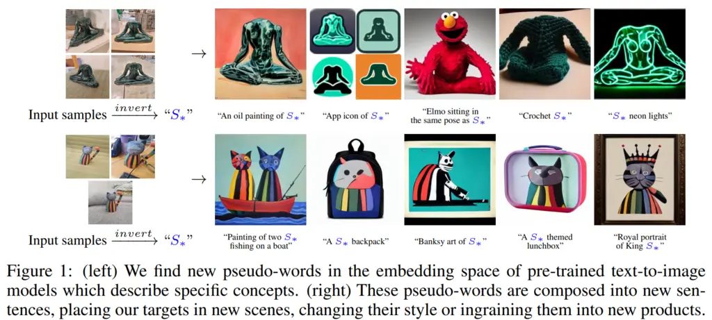
In their approach, they add a new pseudo-word \(S_*\) which represents the user-defined concept. Then the setup, which they call textual inversion works as follows:

  1. Get a few (3-5) images that depicts the concept
  2. The goal is to learn a word embedding of \(S_*\).
  3. Use an optimization process to learn \(S_*\) so that prompts like “a photo of \(S_*\)” will result in images from the training set being generated

A key benefit of their approach is that it does not require fine-tuning the model, which has been associated with catastrophic forgetting of prior knowledge.

2. Optimization Objective

The optimization objective closely resembles that for Latent Diffusion Models (LDMs). Instead of operating in pixel space, LDM operate in the latent space of an autoencoder which has a much lower dimension, hence reducing computational costs significantly.

In diffusion models, the goal is to learn a denoising network that learns the reverse diffusion (noising) process. In other words, given a noised image with a particular noise scale, it learns to remove that noise. This denoising network parameterized by \(\theta\) is denoted by \(\epsilon_\theta\).

In the paper, \(v_*\) is the optimal word embedding to learn for the pseudo-word \(S_*\). Then they give their optimization objective as

\[v_*=\underset{v}{\arg \min } \mathbb{E}_{z \sim \mathcal{E}(x), y, \epsilon \sim \mathcal{N}(0,1), t}\left[\left\|\epsilon-\epsilon_\theta\left(z_t, t, c_\theta(y, v)\right)\right\|_2^2\right],\]

where \(t\) is the time step, \(z_t\) is the latent noised to time step \(t\), and \(c_\theta\) is a model that maps the conditioning input \(y\) and \(v\) into a conditioning vector.

In essence, this objective therefore encourages the network to find the best embedding such that the reconstruction loss from denoising is minimized.

3. Evaluation

They performed qualitative analysis to evaluate their results, and found that it produced results that was closer to the original user-defined concepts than other state-of-the-art approaches.
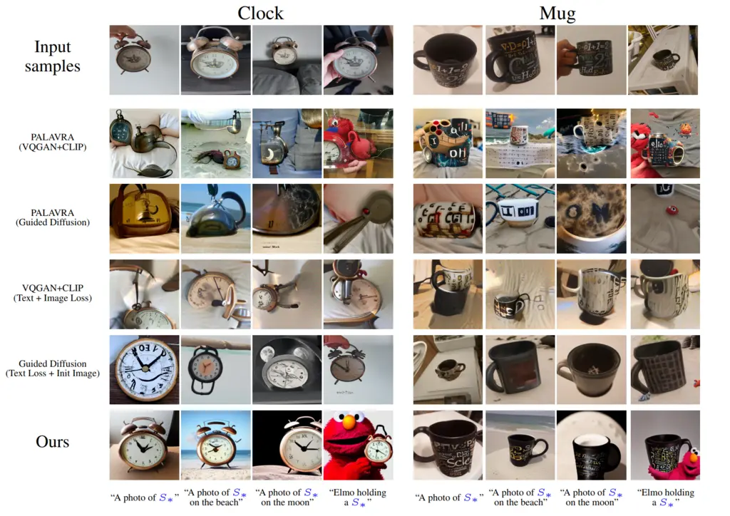
They also performed quantitative analysis using two approaches.

  1. Reconstruction: they generated 64 images using the prompt containing their pseudo-word “A photo of \(S_*\)”. They then took the average pair-wise CLIP-space cosine-similarity between each of the generated images and the user-supplied concept images.

  2. Prompt-adherence: this is measuring how much the generated images adhere to the prompt. This was done by generating a set of images of \(S_*\) with background modifications (“A photo of \(S_*\) on the moon”), style changes (“An oil painting of \(S_*\)”), and compositional relations (“Elmo holding a \(S_*\)”), and then computing the average CLIP embedding over 64 samples. This embedding is then compared to the CLIP embedding of the prompt without \(S_*\) itself, i.e “A photo of on the moon”, by cosine similarity.

Most Glaring Deficiency

Intuitively, it seems like there must be some diversity of the concepts of \(S_*\) supplied (i.e different angles, lighting, levels of zoom) for this to perform well. It would have been interesting to also investigate how the choice of the diversity of the input samples affects the quality of textual inversion.

Conclusions for Future Work

The paper introduces a novel idea of learning an embedding for a visual concept that is hard to express in words, via giving examples of this concept. This idea could be extended to other modalities.