$$ \newcommand{\bone}{\mathbf{1}} \newcommand{\bbeta}{\mathbf{\beta}} \newcommand{\bdelta}{\mathbf{\delta}} \newcommand{\bepsilon}{\mathbf{\epsilon}} \newcommand{\blambda}{\mathbf{\lambda}} \newcommand{\bomega}{\mathbf{\omega}} \newcommand{\bpi}{\mathbf{\pi}} \newcommand{\bphi}{\mathbf{\phi}} \newcommand{\bvphi}{\mathbf{\varphi}} \newcommand{\bpsi}{\mathbf{\psi}} \newcommand{\bsigma}{\mathbf{\sigma}} \newcommand{\btheta}{\mathbf{\theta}} \newcommand{\btau}{\mathbf{\tau}} \newcommand{\ba}{\mathbf{a}} \newcommand{\bb}{\mathbf{b}} \newcommand{\bc}{\mathbf{c}} \newcommand{\bd}{\mathbf{d}} \newcommand{\be}{\mathbf{e}} \newcommand{\boldf}{\mathbf{f}} \newcommand{\bg}{\mathbf{g}} \newcommand{\bh}{\mathbf{h}} \newcommand{\bi}{\mathbf{i}} \newcommand{\bj}{\mathbf{j}} \newcommand{\bk}{\mathbf{k}} \newcommand{\bell}{\mathbf{\ell}} \newcommand{\bm}{\mathbf{m}} \newcommand{\bn}{\mathbf{n}} \newcommand{\bo}{\mathbf{o}} \newcommand{\bp}{\mathbf{p}} \newcommand{\bq}{\mathbf{q}} \newcommand{\br}{\mathbf{r}} \newcommand{\bs}{\mathbf{s}} \newcommand{\bt}{\mathbf{t}} \newcommand{\bu}{\mathbf{u}} \newcommand{\bv}{\mathbf{v}} \newcommand{\bw}{\mathbf{w}} \newcommand{\bx}{\mathbf{x}} \newcommand{\by}{\mathbf{y}} \newcommand{\bz}{\mathbf{z}} \newcommand{\bA}{\mathbf{A}} \newcommand{\bB}{\mathbf{B}} \newcommand{\bC}{\mathbf{C}} \newcommand{\bD}{\mathbf{D}} \newcommand{\bE}{\mathbf{E}} \newcommand{\bF}{\mathbf{F}} \newcommand{\bG}{\mathbf{G}} \newcommand{\bH}{\mathbf{H}} \newcommand{\bI}{\mathbf{I}} \newcommand{\bJ}{\mathbf{J}} \newcommand{\bK}{\mathbf{K}} \newcommand{\bL}{\mathbf{L}} \newcommand{\bM}{\mathbf{M}} \newcommand{\bN}{\mathbf{N}} \newcommand{\bP}{\mathbf{P}} \newcommand{\bQ}{\mathbf{Q}} \newcommand{\bR}{\mathbf{R}} \newcommand{\bS}{\mathbf{S}} \newcommand{\bT}{\mathbf{T}} \newcommand{\bU}{\mathbf{U}} \newcommand{\bV}{\mathbf{V}} \newcommand{\bW}{\mathbf{W}} \newcommand{\bX}{\mathbf{X}} \newcommand{\bY}{\mathbf{Y}} \newcommand{\bZ}{\mathbf{Z}} \newcommand{\calA}{\mathcal{A}} \newcommand{\calB}{\mathcal{B}} \newcommand{\calC}{\mathcal{C}} \newcommand{\calD}{\mathcal{D}} \newcommand{\calE}{\mathcal{E}} \newcommand{\calF}{\mathcal{F}} \newcommand{\calG}{\mathcal{G}} \newcommand{\calH}{\mathcal{H}} \newcommand{\calI}{\mathcal{I}} \newcommand{\calJ}{\mathcal{J}} \newcommand{\calK}{\mathcal{K}} \newcommand{\calL}{\mathcal{L}} \newcommand{\calM}{\mathcal{M}} \newcommand{\calN}{\mathcal{N}} \newcommand{\calO}{\mathcal{O}} \newcommand{\calP}{\mathcal{P}} \newcommand{\calQ}{\mathcal{Q}} \newcommand{\calR}{\mathcal{R}} \newcommand{\calS}{\mathcal{S}} \newcommand{\calT}{\mathcal{T}} \newcommand{\calU}{\mathcal{U}} \newcommand{\calV}{\mathcal{V}} \newcommand{\calW}{\mathcal{W}} \newcommand{\calX}{\mathcal{X}} \newcommand{\calY}{\mathcal{Y}} \newcommand{\calZ}{\mathcal{Z}} \newcommand{\R}{\mathbb{R}} \newcommand{\C}{\mathbb{C}} \newcommand{\N}{\mathbb{N}} \newcommand{\Z}{\mathbb{Z}} \newcommand{\F}{\mathbb{F}} \newcommand{\Q}{\mathbb{Q}} \DeclareMathOperator*{\argmax}{arg\,max} \DeclareMathOperator*{\argmin}{arg\,min} \newcommand{\nnz}[1]{\mbox{nnz}(#1)} \newcommand{\dotprod}[2]{\langle #1, #2 \rangle} \newcommand{\ignore}[1]{} \let\Pr\relax \DeclareMathOperator*{\Pr}{\mathbf{Pr}} \newcommand{\E}{\mathbb{E}} \DeclareMathOperator*{\Ex}{\mathbf{E}} \DeclareMathOperator*{\Var}{\mathbf{Var}} \DeclareMathOperator*{\Cov}{\mathbf{Cov}} \DeclareMathOperator*{\stddev}{\mathbf{stddev}} \DeclareMathOperator*{\avg}{avg} \DeclareMathOperator{\poly}{poly} \DeclareMathOperator{\polylog}{polylog} \DeclareMathOperator{\size}{size} \DeclareMathOperator{\sgn}{sgn} \DeclareMathOperator{\dist}{dist} \DeclareMathOperator{\vol}{vol} \DeclareMathOperator{\spn}{span} \DeclareMathOperator{\supp}{supp} \DeclareMathOperator{\tr}{tr} \DeclareMathOperator{\Tr}{Tr} \DeclareMathOperator{\codim}{codim} \DeclareMathOperator{\diag}{diag} \newcommand{\PTIME}{\mathsf{P}} \newcommand{\LOGSPACE}{\mathsf{L}} \newcommand{\ZPP}{\mathsf{ZPP}} \newcommand{\RP}{\mathsf{RP}} \newcommand{\BPP}{\mathsf{BPP}} \newcommand{\P}{\mathsf{P}} \newcommand{\NP}{\mathsf{NP}} \newcommand{\TC}{\mathsf{TC}} \newcommand{\AC}{\mathsf{AC}} \newcommand{\SC}{\mathsf{SC}} \newcommand{\SZK}{\mathsf{SZK}} \newcommand{\AM}{\mathsf{AM}} \newcommand{\IP}{\mathsf{IP}} \newcommand{\PSPACE}{\mathsf{PSPACE}} \newcommand{\EXP}{\mathsf{EXP}} \newcommand{\MIP}{\mathsf{MIP}} \newcommand{\NEXP}{\mathsf{NEXP}} \newcommand{\BQP}{\mathsf{BQP}} \newcommand{\distP}{\mathsf{dist\textbf{P}}} \newcommand{\distNP}{\mathsf{dist\textbf{NP}}} \newcommand{\eps}{\epsilon} \newcommand{\lam}{\lambda} \newcommand{\dleta}{\delta} \newcommand{\simga}{\sigma} \newcommand{\vphi}{\varphi} \newcommand{\la}{\langle} \newcommand{\ra}{\rangle} \newcommand{\wt}[1]{\widetilde{#1}} \newcommand{\wh}[1]{\widehat{#1}} \newcommand{\ol}[1]{\overline{#1}} \newcommand{\ul}[1]{\underline{#1}} \newcommand{\ot}{\otimes} \newcommand{\zo}{\{0,1\}} \newcommand{\co}{:} %\newcommand{\co}{\colon} \newcommand{\bdry}{\partial} \newcommand{\grad}{\nabla} \newcommand{\transp}{^\intercal} \newcommand{\inv}{^{-1}} \newcommand{\symmdiff}{\triangle} \newcommand{\symdiff}{\symmdiff} \newcommand{\half}{\tfrac{1}{2}} \newcommand{\bbone}{\mathbbm 1} \newcommand{\Id}{\bbone} \newcommand{\SAT}{\mathsf{SAT}} \newcommand{\bcalG}{\boldsymbol{\calG}} \newcommand{\calbG}{\bcalG} \newcommand{\bcalX}{\boldsymbol{\calX}} \newcommand{\calbX}{\bcalX} \newcommand{\bcalY}{\boldsymbol{\calY}} \newcommand{\calbY}{\bcalY} \newcommand{\bcalZ}{\boldsymbol{\calZ}} \newcommand{\calbZ}{\bcalZ} $$

2016

  1. Chiyuan Zhang, Samy Bengio, Moritz Hardt, and 2 more authors
    Nov 2016

    Paper Abstract

    Despite their massive size, successful deep artificial neural networks can exhibit a remarkably small difference between training and test performance. Conventional wisdom attributes small generalization error either to properties of the model family, or to the regularization techniques used during training. Through extensive systematic experiments, we show how these traditional approaches fail to explain why large neural networks generalize well in practice. Specifically, our experiments establish that state-of-the-art convolutional networks for image classification trained with stochastic gradient methods easily fit a random labeling of the training data. This phenomenon is qualitatively unaffected by explicit regularization, and occurs even if we replace the true images by completely unstructured random noise. We corroborate these experimental findings with a theoretical construction showing that simple depth two neural networks already have perfect finite sample expressivity as soon as the number of parameters exceeds the number of data points as it usually does in practice. We interpret our experimental findings by comparison with traditional models.

Three Important Things

1. Deep Neural Networks Easily Fit Random Labels

It is an open problem as to why over-parameterized neural networks can generalize well even in the absence of regularization, as conventional wisdom would lead us to believe it should overfit to the training data.

To this end, people have applied classical learning theories like VC (Vapnik–Chervonenkis) dimension, Rademacher complexity, and uniform stability to argue that if the complexity of the network is bounded in some way, then it will generalize and not overfit. Specifically:

  1. VC dimension: the VC dimension of a classifier is the largest number of points that it can classify correctly, for all possible assignments of their labels. So a classifier with VC dimension \(n\) can perfectly fit any labeling of \(n\) datapoints.

  2. Rademacher complexity: the Rademacher complexity \(\hat{\mathfrak{R}}_n(\mathcal{H})\) on a hypothesis class \(\mathcal{H}\) on \(n\) datapoints \(x_1, \cdots, x_n\) is defined as

    \[\hat{\mathfrak{R}}_n(\mathcal{H})=\mathbb{E}_\sigma\left[\sup _{h \in \mathcal{H}} \frac{1}{n} \sum_{i=1}^n \sigma_i h\left(x_i\right)\right],\]

    where \(\sigma\) is drawn according to an \(n\)-dimensional \(\{-1, +1\}\) Rademacher distribution, and we can think of the supremum \(h\) for each \(\sigma\) as the function in the function class that can best fit each \(h(x_i)\) to the labels \(\sigma_i\) such that the sum is maximized. In other words, it is the capacity of the function class in fitting the data to random labels.

    Trivially, a Rademacher complexity of 1 given the \(n\) datapoints means the function class is large enough to fit all random labelings.

  3. Uniform stability: uniform stability captures the notion that the predictions of a classifier does not change too much when only a single example is removed or perturbed. A classifier \(f\) is \(\beta\)-uniformly stable with respect to some loss \(\ell\) if for any two datasets \(S, S'\) that only differ in a training example, then the difference in their losses is bounded by \(\beta\) for any input-label pair \((x,y)\), we have:

    \[|\ell(f_S(x), y) - \ell(f_{S'}(x), y)| < \beta,\]

    where \(f_S\) and \(f_{S'}\) are the classifier trained on \(S\) and \(S'\) respectively.

The authors found that standard neural network architectures like Inception V3 on popular benchmark datasets like CIFAR10 could fit random assignment of training labels, and also other forms of corruption of the data:
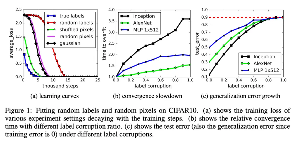
This shows that the VC dimension of the network is probably larger than the dataset, and that the Rademacher complexity is close to one. If their complexities are so large then any theory based on it to show some regularization property to help in demonstrating how it generalizes is essentially useless.

Hence, alternative frameworks for thinking about generalization for large networks beyond standard learning theory concepts are required.

2. Explicit Regularization Helps, But Is Not Necessary For Generalization

Since implicit regularization (if any) of the networks was clearly not enough to restrict its expressiveness to fit any random data, what if we introduced explicit regularization such as dropout, weight-decay, and batchnorm?

Unfortunately, even with regularization the various popular architectures were still able to almost perfectly fit random labels:
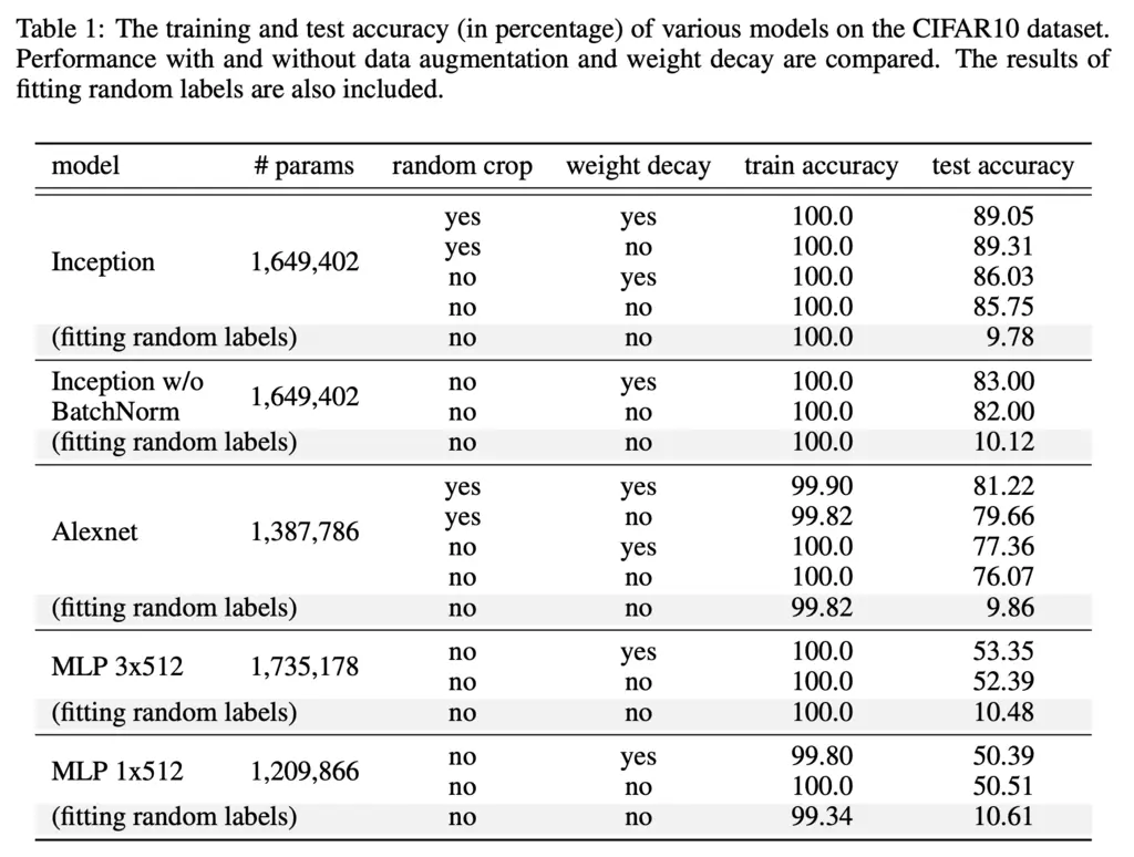
Note that since CIFAR10 has 10 classes, random guessing gives 10% accuracy and hence fitting random labels predictably performed no better than random guessing.

In addition, even in the absence of any explicit regularization, it could also generalize well and have test accuracy almost on-par to when explicit regularization was enabled.

This shows that explicit regularization can help, but is not essential for generalization.

3. Finite-Sample Expressivity

The fact that all our popular neural networks can memorize training labels perfectly might feel a bit shocking or even depressing.

It might then be worth asking just how big (or small) a neural network must be before it is capable of such memorizing.

Traditionally, people answered this by attempting to find the function class that a neural network with a certain number of parameters can express. However, the authors take a different and much simpler approach by asking instead how large a neural network must be to memorize \(n\) samples. This led to their main theoretical result in the paper:

Theorem (Neural Networks Of Size Linear To Sample Size Sufficient For Memorization)
There exists a two-layer neural network with ReLU activations and \(2n+d\) weights that can represent any function on a sample of size \(n\) in \(d\) dimensions.

Most Glaring Deficiency

In all honesty, I thought this was a very interesting and well-written paper considering the first author did it while interning at Google Brain (in contrast I feel that I accomplished nothing as cool or novel during my own internships).

However, I must say that I would be surprised if no one realized that neural networks are capable of fitting random labels before this paper. I’m very positive that by the way of a programming bug or otherwise, someone should have already discovered this phenomenon way before, but probably did not think a lot about the ramifications of this fact.

In addition, it might have been interesting to explore how removing known inductive bias that helps a particular problem domain may affect generalization. For instance, instead of using CNNs with strong inductive bias for visual data, it may have been interesting to see how the results would change if regular neural networks were used instead.

Conclusions for Future Work

Understanding generalization of over-parameterized models requires us to go beyond classical learning theory and explore alternative ways of studying the models, since these models are so over-parameterized and expressive that these theories would only ever be able to produce trivial bounds.