$$ \newcommand{\bone}{\mathbf{1}} \newcommand{\bbeta}{\mathbf{\beta}} \newcommand{\bdelta}{\mathbf{\delta}} \newcommand{\bepsilon}{\mathbf{\epsilon}} \newcommand{\blambda}{\mathbf{\lambda}} \newcommand{\bomega}{\mathbf{\omega}} \newcommand{\bpi}{\mathbf{\pi}} \newcommand{\bphi}{\mathbf{\phi}} \newcommand{\bvphi}{\mathbf{\varphi}} \newcommand{\bpsi}{\mathbf{\psi}} \newcommand{\bsigma}{\mathbf{\sigma}} \newcommand{\btheta}{\mathbf{\theta}} \newcommand{\btau}{\mathbf{\tau}} \newcommand{\ba}{\mathbf{a}} \newcommand{\bb}{\mathbf{b}} \newcommand{\bc}{\mathbf{c}} \newcommand{\bd}{\mathbf{d}} \newcommand{\be}{\mathbf{e}} \newcommand{\boldf}{\mathbf{f}} \newcommand{\bg}{\mathbf{g}} \newcommand{\bh}{\mathbf{h}} \newcommand{\bi}{\mathbf{i}} \newcommand{\bj}{\mathbf{j}} \newcommand{\bk}{\mathbf{k}} \newcommand{\bell}{\mathbf{\ell}} \newcommand{\bm}{\mathbf{m}} \newcommand{\bn}{\mathbf{n}} \newcommand{\bo}{\mathbf{o}} \newcommand{\bp}{\mathbf{p}} \newcommand{\bq}{\mathbf{q}} \newcommand{\br}{\mathbf{r}} \newcommand{\bs}{\mathbf{s}} \newcommand{\bt}{\mathbf{t}} \newcommand{\bu}{\mathbf{u}} \newcommand{\bv}{\mathbf{v}} \newcommand{\bw}{\mathbf{w}} \newcommand{\bx}{\mathbf{x}} \newcommand{\by}{\mathbf{y}} \newcommand{\bz}{\mathbf{z}} \newcommand{\bA}{\mathbf{A}} \newcommand{\bB}{\mathbf{B}} \newcommand{\bC}{\mathbf{C}} \newcommand{\bD}{\mathbf{D}} \newcommand{\bE}{\mathbf{E}} \newcommand{\bF}{\mathbf{F}} \newcommand{\bG}{\mathbf{G}} \newcommand{\bH}{\mathbf{H}} \newcommand{\bI}{\mathbf{I}} \newcommand{\bJ}{\mathbf{J}} \newcommand{\bK}{\mathbf{K}} \newcommand{\bL}{\mathbf{L}} \newcommand{\bM}{\mathbf{M}} \newcommand{\bN}{\mathbf{N}} \newcommand{\bP}{\mathbf{P}} \newcommand{\bQ}{\mathbf{Q}} \newcommand{\bR}{\mathbf{R}} \newcommand{\bS}{\mathbf{S}} \newcommand{\bT}{\mathbf{T}} \newcommand{\bU}{\mathbf{U}} \newcommand{\bV}{\mathbf{V}} \newcommand{\bW}{\mathbf{W}} \newcommand{\bX}{\mathbf{X}} \newcommand{\bY}{\mathbf{Y}} \newcommand{\bZ}{\mathbf{Z}} \newcommand{\calA}{\mathcal{A}} \newcommand{\calB}{\mathcal{B}} \newcommand{\calC}{\mathcal{C}} \newcommand{\calD}{\mathcal{D}} \newcommand{\calE}{\mathcal{E}} \newcommand{\calF}{\mathcal{F}} \newcommand{\calG}{\mathcal{G}} \newcommand{\calH}{\mathcal{H}} \newcommand{\calI}{\mathcal{I}} \newcommand{\calJ}{\mathcal{J}} \newcommand{\calK}{\mathcal{K}} \newcommand{\calL}{\mathcal{L}} \newcommand{\calM}{\mathcal{M}} \newcommand{\calN}{\mathcal{N}} \newcommand{\calO}{\mathcal{O}} \newcommand{\calP}{\mathcal{P}} \newcommand{\calQ}{\mathcal{Q}} \newcommand{\calR}{\mathcal{R}} \newcommand{\calS}{\mathcal{S}} \newcommand{\calT}{\mathcal{T}} \newcommand{\calU}{\mathcal{U}} \newcommand{\calV}{\mathcal{V}} \newcommand{\calW}{\mathcal{W}} \newcommand{\calX}{\mathcal{X}} \newcommand{\calY}{\mathcal{Y}} \newcommand{\calZ}{\mathcal{Z}} \newcommand{\R}{\mathbb{R}} \newcommand{\C}{\mathbb{C}} \newcommand{\N}{\mathbb{N}} \newcommand{\Z}{\mathbb{Z}} \newcommand{\F}{\mathbb{F}} \newcommand{\Q}{\mathbb{Q}} \DeclareMathOperator*{\argmax}{arg\,max} \DeclareMathOperator*{\argmin}{arg\,min} \newcommand{\nnz}[1]{\mbox{nnz}(#1)} \newcommand{\dotprod}[2]{\langle #1, #2 \rangle} \newcommand{\ignore}[1]{} \let\Pr\relax \DeclareMathOperator*{\Pr}{\mathbf{Pr}} \newcommand{\E}{\mathbb{E}} \DeclareMathOperator*{\Ex}{\mathbf{E}} \DeclareMathOperator*{\Var}{\mathbf{Var}} \DeclareMathOperator*{\Cov}{\mathbf{Cov}} \DeclareMathOperator*{\stddev}{\mathbf{stddev}} \DeclareMathOperator*{\avg}{avg} \DeclareMathOperator{\poly}{poly} \DeclareMathOperator{\polylog}{polylog} \DeclareMathOperator{\size}{size} \DeclareMathOperator{\sgn}{sgn} \DeclareMathOperator{\dist}{dist} \DeclareMathOperator{\vol}{vol} \DeclareMathOperator{\spn}{span} \DeclareMathOperator{\supp}{supp} \DeclareMathOperator{\tr}{tr} \DeclareMathOperator{\Tr}{Tr} \DeclareMathOperator{\codim}{codim} \DeclareMathOperator{\diag}{diag} \newcommand{\PTIME}{\mathsf{P}} \newcommand{\LOGSPACE}{\mathsf{L}} \newcommand{\ZPP}{\mathsf{ZPP}} \newcommand{\RP}{\mathsf{RP}} \newcommand{\BPP}{\mathsf{BPP}} \newcommand{\P}{\mathsf{P}} \newcommand{\NP}{\mathsf{NP}} \newcommand{\TC}{\mathsf{TC}} \newcommand{\AC}{\mathsf{AC}} \newcommand{\SC}{\mathsf{SC}} \newcommand{\SZK}{\mathsf{SZK}} \newcommand{\AM}{\mathsf{AM}} \newcommand{\IP}{\mathsf{IP}} \newcommand{\PSPACE}{\mathsf{PSPACE}} \newcommand{\EXP}{\mathsf{EXP}} \newcommand{\MIP}{\mathsf{MIP}} \newcommand{\NEXP}{\mathsf{NEXP}} \newcommand{\BQP}{\mathsf{BQP}} \newcommand{\distP}{\mathsf{dist\textbf{P}}} \newcommand{\distNP}{\mathsf{dist\textbf{NP}}} \newcommand{\eps}{\epsilon} \newcommand{\lam}{\lambda} \newcommand{\dleta}{\delta} \newcommand{\simga}{\sigma} \newcommand{\vphi}{\varphi} \newcommand{\la}{\langle} \newcommand{\ra}{\rangle} \newcommand{\wt}[1]{\widetilde{#1}} \newcommand{\wh}[1]{\widehat{#1}} \newcommand{\ol}[1]{\overline{#1}} \newcommand{\ul}[1]{\underline{#1}} \newcommand{\ot}{\otimes} \newcommand{\zo}{\{0,1\}} \newcommand{\co}{:} %\newcommand{\co}{\colon} \newcommand{\bdry}{\partial} \newcommand{\grad}{\nabla} \newcommand{\transp}{^\intercal} \newcommand{\inv}{^{-1}} \newcommand{\symmdiff}{\triangle} \newcommand{\symdiff}{\symmdiff} \newcommand{\half}{\tfrac{1}{2}} \newcommand{\bbone}{\mathbbm 1} \newcommand{\Id}{\bbone} \newcommand{\SAT}{\mathsf{SAT}} \newcommand{\bcalG}{\boldsymbol{\calG}} \newcommand{\calbG}{\bcalG} \newcommand{\bcalX}{\boldsymbol{\calX}} \newcommand{\calbX}{\bcalX} \newcommand{\bcalY}{\boldsymbol{\calY}} \newcommand{\calbY}{\bcalY} \newcommand{\bcalZ}{\boldsymbol{\calZ}} \newcommand{\calbZ}{\bcalZ} $$

2018

  1. Simon S. Du, Xiyu Zhai, Barnabas Poczos, and 1 more author
    Oct 2018

    Paper Abstract

    One of the mysteries in the success of neural networks is randomly initialized first order methods like gradient descent can achieve zero training loss even though the objective function is non-convex and non-smooth. This paper demystifies this surprising phenomenon for two-layer fully connected ReLU activated neural networks. For an m hidden node shallow neural network with ReLU activation and n training data, we show as long as m is large enough and no two inputs are parallel, randomly initialized gradient descent converges to a globally optimal solution at a linear convergence rate for the quadratic loss function. Our analysis relies on the following observation: over-parameterization and random initialization jointly restrict every weight vector to be close to its initialization for all iterations, which allows us to exploit a strong convexity-like property to show that gradient descent converges at a global linear rate to the global optimum. We believe these insights are also useful in analyzing deep models and other first order methods.

Three Important Things

1. Wide Two-Layer Neural Networks with Gram Matrix Spectral Properties Enjoys Linear Convergence Rate

This paper shows theoretically how overparameterization of a two-layer neural network can result in a linear rate of convergence (linear when logarithms are taken, hence it really converges exponentially fast).

The setup of the paper is a standard two-layer neural network of the following form:

\[f(\mathbf{W}, \mathbf{a}, \mathbf{x})=\frac{1}{\sqrt{m}} \sum_{r=1}^{m} a_{r} \sigma\left(\mathbf{w}_{r}^{\top} \mathbf{x}\right)\]

The first layer is initialized with random Gaussians, and the second layer is initialized uniformly with either -1 or +1. The reason \(\pm 1\) initialization was used in the second layer is because it simplifies the Gram matrix of the weights.

The Gram matrix \(\bH\) referred to in the paper is defined as the matrix product of the differential map of \(f\) with its transpose, i.e \(\nabla_W f \, \nabla_W f^{\top}\). This is similar to the kernel in the neural tangent kernel paper. Note that the eigenvalues of the Gram matrix are always non-negative since the Gram matrix is positive semi-definite.

The main result of the paper states that if the following conditions hold:

  1. The neural network is initialized in the manner mentioned previously,
  2. The Gram matrix \(\bH\) induced by ReLU activation and random initialization has its smallest eigenvalue \(\lambda_0\) bounded away from 0 (this is the key assumption used),
  3. We set step size \(\eta = O \left( \frac{\lambda_0}{n^2} \right)\),
  4. The number of hidden notes is at least \(m = \Omega \left( \frac{n^6}{ \lambda_0^4 \delta^3 } \right)\),

then with probability at least \(1-\delta\) over the random initializations, we have that for any time step \(k\), the difference between the output of the network \(\bu(k)\) and the labels \(\by\) can be bounded:

\[\| \bu(k) - \by \|_2^2 \leq \left( 1 - \frac{\eta \lambda_0}{2} \right)^k \| \bu(0) - \by \|_2^2.\]

In other words, it converges at a linear rate.

2. Spectral Norm of Gram Matrix Does Not Change Much During Gradient Descent

An essential part of the proof in the main theorem requires that the smallest eigenvalue assumption of the Gram matrix \(\bH\) holds throughout gradient descent. They showed this by first showing that the randomly initialized \(\bH(0)\) at time step 0 is close in spectral norm to \(\bH^{\infty}\), defined as

\[\mathbf{H}_{i j}^{\infty}= \mathbb{E}_{\mathbf{w} \sim N(\mathbf{0}, \mathbf{I})}\left[\mathbf{x}_{i}^{\top} \mathbf{x}_{j} \mathbb{I}\left\{\mathbf{w}^{\top} \mathbf{x}_{i} \geq 0, \mathbf{w}^{\top} \mathbf{x}_{j} \geq 0\right\}\right].\]

Precisely, they showed that if \(m\) is wide enough, then with high probability, \(\left\|\mathbf{H}(0)-\mathbf{H}^{\infty}\right\|_{2} \leq \frac{\lambda_{0}}{4}\) and \(\lambda_{\min }(\mathbf{H}(0)) \geq \frac{3}{4} \lambda_{0}\).

They then used this result to show that any \(\bH(t)\) is stable, and is close to its value at initialization.

3. Synthetic Data To Validate Theoretical Findings
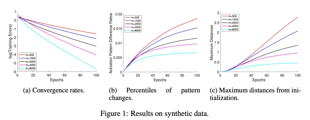
The authors generated synthetic data to verify their theoretical findings. They found that:

  1. Greater widths result in faster convergence,
  2. Greater widths result in fewer activation pattern changes, which verifies the stability of the Gram matrix,
  3. Greater widths result in smaller weight changes.

Most Glaring Deficiency

The assumption that the second layer of the neural networks is initialized with \(\pm 1\) values feels quite unrealistic, although it is admittedly to simplify the theoretical analysis. It would be interesting to see if such an initialization pattern could actually be competitive with established weight initialization techniques in practice.

Conclusions for Future Work

Their work provides a further stepping stone to understanding why over-parameterized models perform so well. As the authors mentioned, it may be possible to generalize the results of their approach to deeper neural networks.