Dynamic Programming | हृषीकेश सिंह

Objective : Assuming this as a first writeup of the series, the aim is to set the foundation of Dynamic Programming fundamentals along with a generic framework to disintegrate any coding interview problem into components.

1. Pre-Requisites

Fundamental understanding of Recurrence relation, Divide & Conquer methodology and especially DFS traversal.
Time $(Big-O)$ and Space complexities of Recurrence Relation. (Master Theorem)
Operations based on Arrays & List.
Basic Understanding of Matrix traversals.

2. Basic Foundation

2.1 Introduction

What does word “Dynamic” signifies in Dynamic Programming ?

Well actual history is that, DP was invented by Richard Bellman (pre-cursor to Bellman Ford Algorithm) and he claimed that he invented Dynamic Programming to hide the fact that he was doing mathematical research. He was working at RAND under a Secretary of Defence who had a pathological fear towards the word “research” so he settled on the term “Dynamic” since it will be difficult to give meaning to it and not even a congressman could object to it. Basically it sounded cool.

For a conceptual understanding, let’s start with a classical example of Fibonacci Numbers.

For given $F(n)$, return the value for any given n.

\[\displaylines{ F(n) = \begin{cases} 0, & \text{if $n = 0$}\\ 1, & \text{if $n = 1$}\\ F(n - 1) + F(n - 2), & \text{if $n > 1$} \end{cases} }\]

Then Subproblem graph for Fibonacci will be :-

  graph TB
      F4[4] --> F3[3]
      F4[4] --> F2[2]
      F3[3] --> F1[1]
      F3[3] --> F2[2]
      F2[2] --> F1[1]
      F2[2] --> F0[0]

A naive approach if translated into a recursive code will be :

  public int fibonacci(int n){
  	if(n == 1 || n == 0){
  	  return n;
  	}
    return fibonacci(n-1) + fibonacci(n-2);
  }

What will be the time complexity of this naive recursive code ?

An initial assumption might be that it is $O(2^n)$, as it is a recursive formula that branches twice each call, but this isn’t the best upper-bound.

The complexity of fibonacci is $O(Fn) = O(ϕ^n)$. This is approximately $O(1.618^n)$. Still awful, but a little better than the initial assumption of $O(2^n)$.

But if you closely notice in the function call tree, the computations are being re-done and hence adding complexities. These computations could be avoided by storing the computed values and reusing it futher. For example a simpler iterative solution of this problem :-
```
  public int fibonacciIterative(int n){
  	int n1 = 0, n2 = 1;
    int sum;
    
    if (n == n1 || n == n2)    return n;
    	
  	for(int i=2; i <= n; i++){
  	  sum = n1 + n2;
  	  n1 = n2;
      n2 = sum;
    }
  	return n2;
  }
```
What will be the time complexity of this simpler iterative code ? (✅ Test)

Time complexity $\approx O(n)$

How to distinct divide and conquer from dynamic programming?

In divide and conquer, problems are divided into disjoint subproblems, the subproblem graph would degrade to a tree structure, each subproblem other than the base problems (here it is each individual element in the array) will only have out degree equals to 1. (e.g. Merge sort function call tree).

In comparison, in the case of fibonacci sequence, some problems would have out degree larger than one, which makes the network a graph instead of a tree structure. This characteristics is directly induced by the fact that the subproblems overlap – that is, subproblems share subprolems. For example, f(4) and f(3) share f(2), and f(3) and f(2) shares f(1).

💡 Dynamic programming is simplifying a complicated problem by breaking it down into simpler sub-problems in a recursive manner.

2.2 Why it is required ?

Dynamic programming is an optimization methodology over the complete search solutions for typical optimization problems. Dynamic Programming’s core principle is to solve each subproblem only once by saving and reusing its solution. Therefore, comparing with its naive counterpart – Complete Search:

Dynamic Programming avoids the redundant recomputation met in its compete search counterpart as demonstrated in the last section.
Dynamic Programming uses additional memory as a trade-off for better computation/time efficiency; it serves as an example of a time-space trade-off. In most cases, the space overhead is well-worthy; it can decrease the time complexity dramatically from exponential $O(K^n)$ to polynomial level $O(n)$.

2.3 Where can it be implemented?

Dynamic programming problems are normally asked in its certain way and its naive solution shows certain time complexity (mostly exponential). So for a clear understanding I would like to put it this way which is way more simpler thant textbooks by providing the situations when to use or not to use dynamic programming as Do’s and Do-nots.

Do’s : Dynamic programming fits for the optimizing the following problems which are either exponential or polynomial complexity using complete search :-

Optimization: Compute the maximum or minimum value;
Counting: Count the total number of solutions;
Checking if a solution work

Do Nots : In the following cases we might not be able to apply Dynamic Programming:

When the naive solution has a low time complexity already such as $O(n^2)$ or $O(n^3)$.
When the input dataset is a set while not an array or string or matrix, 90% chance we will not use DP.
When the overlapping subproblems apply but it is not optimization problems thus we can not identify the suboptimial substructure property and thus find its recurrence function. For example, same problem context as in Dos but instead we are required to obtain or print all solutions, this is when we need to retreat back to the use of DFS+memo(top-down) instead of DP.

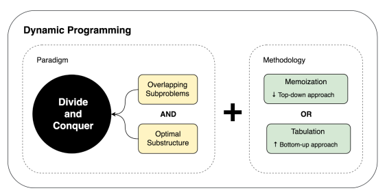
2.4 How can it be implemented/approached ?

💡 Note : While teaching, the educator should give a bird eye overview about the two possible approaches to students so that they can have a mental framework to place the details mentioned in Illustration section later.

In this section, we have provided two forms of dynamic programming solutions: memoization and tabulation, as two different ways of bringing the caching mechanism into practice. In this section, we focus on the iterative tabulation and generalize its four key elements and practical guidelines for importants steps.

Dynamic programming for optimizing the problems fall into the broadly three categories:
1. Optimization: Compute the maximum or minimum value;
2. Counting: Count the total number of solutions;
3. Checking if a solution works or not, True or False;
Now to fit in the above 3 categories, the problem must show 2 essential properties :
- Overlapping subproblems.
- Optimal substructures.

Before understanding the approach, we must get familiar with these two properties of the subproblems : -

What are Overlapping Subproblems ?

When a recursive algorithm revisits the same subproblem repeatedly, we say that the optimization problem has overlapping subproblems. where one subproblem is reached by multiple other subproblem. When subproblems are disjoint such as seen in merge sort and binary search, dynamic programming would not be helping.
Optimal Substructure

A given problem has optimal substructure property if the optimal solution of the given problem can be obtained by using optimal solutions of its subproblems. Only if optimal substructure property applied we can find the recurrence relation function which is a key step in implementation as we have seen from the above two examples. Optimal substructures varies across problem domains in two ways:
1. Subproblem space: how many subproblems an optimal solution to the original problem uses. For example, in Fibonacci sequence, each integer in range [0, n] is a subproblem, which makes the n + 1 as the total subproblem space. The state of each subproblem is the optimal solution for that subproblem which is f(n).
2. State Choice: how many choices we have in determining which subproblem(s) to use to decide the recurrence function for the current state. In Fibonacci sequence, each state only relies on two preceding states as seen in recurrence function f(i) = f(i − 1) + f(i − 2), thus making it constant cost.
  
  Subproblem space and state choice together not only formulates the recurrent relation with which we very much have the implementation in hand. Together they also decide the time and space complexity we will need to tackle our dynamic programming problems

Two Forms of Dynamic Programming Solution

There are two ways either recursive or iterative in general to add space mechanism into naive complete search to construct our dynamic programming solution.

💡 But do remember that we cannot eliminate recursive thinking completely. We will always have to define a recursive relation irrespective of the approach we use.

Design

Top-down + Memoization (recursive DFS)

We start from larger problem (from top) and recursively search the subproblems space (to bottom) until the leaf node. This method is built on top of Depth-First Graph Search together with Divide and Conquer Methodology which treat each node as a subproblem and return its solution to its caller so that it can be used to build up its solution.

Following a top-down fashion as is in divide and conquer, along the process, in the recursive call procedure, a hashmap is relied on to save and search solutions. The memoization works in such way that at the very first time that the subproblem is solved it will be saved in the hashmap, and whenever this problem is met again, it finds the solution and returns it directly instead of computing again.

The key elements of this style of dynamic programming is:
1. Define subproblem;
2. Develop solution using Depth-first Graph search and Divide and conquer (leave alone the recomputation).
3. Adding hashmap to save and search the state of each subproblem

Bottom-up + Tabulation (iterative)

Different from the last method, which use recursive calls, in this method, we approach the subproblems from the smallest subproblems, and construct the solutions to larger subproblems using the tabulaized result. The nodes in the subproblem graph is visited in a reversed topological sort order. This means that to reconstruct the state of current subproblem, all dependable (predecessors) have already be computed and saved.
- The memoization method applies better for beginners that who have decent understanding of divide and conquer. However, once you have enough practice, the tabulation should be more intuitive compared with recursive solution. Usually, dynamic programming solution to a problem refers to the solution with tabulation.

Five Steps to Solve Dynamic Programming

This is a general guideline for dynamic programming – memoization or tabulation. Key advice – being “flexbile”.

Given a real problem, all in all, we are credited with our understanding of the concepts in computer science. Thus, we should not be too bothered or stressed that if you can not come up with a “perfect” answer.

Step 1 : Read the question: search for the key words of the problem patterns: counting, checking, or maximum/minimum.
Step 2 : Come up with the most naive solution ASAP: analyze its time complexity. Is it a typical DFS solution? Try draw a SUBPROBLEM GRAPH to get visualization. Is there space for optimization?
Step 3 : Is there overlapping? Can you define the optimal substructure/recurrence function?
Step 4 : If the conclusion is YES, try to define the Five key elements so that we can solve it using the preferable tabulation. If you can figure it out intuitively just like that, great! What to do if not? Maybe retreat to use memoization, which is a combination of divide and conquer, DFS, and memoization.
Step 5. What if we were just so nervous that or time is short, we just go ahead and implement the complete search solution instead. With implementation is better than nothing. With the implementation in hand, maybe we can figure it out later.

Five Key Elements of Tabulation

As the first guideline of Tabulation, we summarize the four key elements for the implementation of dynamic programming:

Step 4.1 : Subproblem and State

Define what the subproblem space, what is the optimal state/solution for each subproblem. In practice, it would normally be the the total/the maximum/minimum for subproblem. This requires us to know how to divide problem into subproblems.
Step 4.2 : State Transfer (Recurrence) Function:

Derive the function that how we can get current state by using result from previous computed state(s). This requires us to identify the optimal substructure and know how to make state choice.
Step 4.3 : Assignment and Initialization:

Followed by knowing the subproblem space, we typically assign a space data structure and initialize its values. For base or edge cases, we might need to initialize different than the other more general cases
Step 4.4 : Iteration:

Decide the order of iterating through the subproblem space thus we can scan each subproblem/state exact and only once. Using the subproblem graph, and visit the subproblms in reversed topological order is a good way to go.
Step 4.5 : Answer:

Decide which state or a combination of all states such as the the max/min of all the state is the final result needed.

Complexity Analysis

The complexity analysis of the tabulation is seemingly more straightforward compared with its counterpart – the recursive memoization. For the tabulation, we can simply draw conclusion without any prior knowledge of the dynamic programming by observing the for loops and its recurrence function. However, for both variant, there exists a common analysis method.
The core points to analyze complexity involving dynamic programming is:
1. The subproblem space |S|, that is the total number of subproblems; and
2. The number of state choice needed to construct each state |C|.
By multiplying these two points, we can draw the conclusion of its time complexity as O(|S|.|C|).
For example, if the subproblem space is n and if each state i relies on
1. Only one or two previous states as we have seen in the example of Fibonacci Sequence, it makes the time complexity O(n); and
2. All previous states in range [0, i − 1] as seen in the example of Longest Increasing Subsequence, which can be viewed as $O(n)$ to solve each subproblem, this brings up the complexity up to $O(n^2)$.

To help you decide which style that you should take when presented with a DP solution, here’s the trade-off comparison between top-down Memoization and bottom-up Tabulation

	Memoization	Tabulation
Pros	1. A natural transformation from normal recursive complete search. 2. Compute subproblems only when necessary, sometimes this can be faster.	1. Faster if many sub-problems are revisited as there is no overhead of recursive calls. 2. Can save memory space with dynamic programming ‘on-the-fly’ technique.
Cons	1. Slower if many subproblems are revisited due to overhead of recursive calls. 2. If there are n states, it can use up to O(n) table size which might lead to Memory Limit Exceeded(MLE) for some hard problems. 3. Faces stack overflow due to the recursive calls.	1. For programmers who are inclined with recursion, this may not be intuitive.

2.5 Illustration

For a details illustration, let’s start with one of the generic parent problem called Knapsack Problem. This problem type gives the foundational aspect for other variants too. Hence a deeper understanding of this problem type is required for understanding the inner working of Dynamic Programming.

💡 The Knapsack problem, as the name suggests, is the problem faced by a person who has a knapsack with a limited capacity and wants to carry the most valuable items. In other words, we are given N items, each having a specific weight and a value, and a knapsack with a maximum capacity.

Our job is to put as many items as possible in the knapsack such that the cumulative weight of the items doesn’t exceed the knapsack’s capacity, and the cumulative value of the items in the knapsack is maximized.

Problem statement : The 0/1 Knapsack is a special case of the Knapsack problem where item selection has some constraints. In general, the following restrictions are applied:

A maximum of one item can be selected of each kind, that is, the number of items of each kind in the knapsack is either zero or one.
We can’t take a fraction of an item, that is, we either have to take the complete item or leave it.

💡 Mathematically, Given a set of n items, each with a value $v_i$ and weight $w_i$, and a knapsack with maximum weight capacity C , we have the following target:

\[Maximize \sum_{i=1}^n x_i v_i\] \[Subject~~to \sum_{i=1}^n x_i v_i \ \leq C\]

with $x_i ∈ \{0,1\}$ representing the number of instances of item i in the knapsack.

Before proceeding, let’s check if the students have understood the problem statement type. Here are few problem statements, let’s see if these are 0/1 Knapsack problem type or other types.
- Given a set of positive numbers, find a triplet whose sum is equal to a given number S (✅ 0/1 Knapsack)
- Select one car of each model to be displayed in the showroom so that the overall worth of the displayed cars is maximized. (✅ 0/1 Knapsack)
- Given an unlimited number of tennis balls, calculate the number of balls that can be placed in a box. (❌ Other type)
- Given an array of numbers, calculate the number of ways in which its elements can be selected to make sum S. (❌ Other type)
- Plan a vacation in such a way that the maximum number of cities is visited in the specified budget. (✅ 0/1 Knapsack)

Let’s start solving the problem with our proposed Five Step Framework from section 2.4

Step 1 - 3

Search for keyword aiming for optimization : Maximize the value of whole knapsack.
Start with Naive Solution just to get an approximate idea of time complexity and the typical DFS approach. It will be a good idea to start with Subproblem graph.
Check for overlapping subproblems : Yes.
Can a recurrence relation be defined among subproblems : Yes.

Step 4

Now we have two options here to proceed with : Memoization or Tabulation. Let’s first explore the Tabulation Approach :-

Step 4.3 : Assignment and Initialization

Assign a space datastructure and initialize its base, edge and normal values.
Since this is profit maximizing problem hence the least amount of profit in case of a null set or null capacity will 0. Moreover we will have to take an extra row and column to consider this condition.

  // Initialize a table where individual rows represent items
  // and columns represent the weight of the knapsack
    
  final int N = W.length;
    
  //Extra row and coloums are taken to consider the empty set condition.
  int[][] DP = new int[N + 1][capacity + 1];
    
  for(int i = 0; i < N+1; i++){
  	for(int j = 0; j < capacity+1; j++){
  		if( i == 0 || j == 0)  DP[i][j] = 0;
  	}
  }

Step 4.4 : Iteration

Determine the order of iterating through subproblem space to avoid repeated computation hence visiting the subproblem in a reverse topological order (bottom up) is a good way to go.

  		public int bottomUpDP(int val[], int wt[], int capacity){
          final int N = wt.length;
  				int DP[][] = new int[N + 1][capacity + 1];
    
          for(int i = 0; i < N + 1; i++){
              for(int j = 0; j < W + 1; j++){
                  if(i == 0 || j == 0){
                      DP[i][j] = 0;
                      continue;
                  }
                  if(j - wt[i-1] >= 0){
                      DP[i][j] = Math.max(DP[i-1][j], DP[i-1][j-wt[i-1]] + val[i-1]);
                  }else{
                      DP[i][j] = DP[i-1][j];
                  }
              }
          }
          return DP[N][capacity];
      }

Step 4.5 : Answer
- Final result will be stored at the $DP[N][capacity]$ since this value allows for all the items to be considered for the maximum possible capacity. Hence this is the answer.

The above elaboration might have given you a fair idea of the approach. Now let’s say you have a knapsack capacity of 5 and a list of items with weights and values as follows:

\[weights = [1, 2, 3, 5] ~~~~~~~~~~~~~~~~values = [10, 5, 4, 8]\]

There are four ways of storing items in the knapsack, such that the combined weight of stored items is less than or equal to the knapsack’s capacity.

Item of weight 1 and weight 2, with a total value of 15.
Item of weight 1 and weight 3, with a total value of 14.
Item of weight 2 and weight 3, with a total value of 9.
Item of weight 5, with a value of 8.

Though all of the combinations described above are valid, we need to select the one with the maximum value. Hence, we will select items with weights 1 and 2, as they give us the maximum value of 15.

Constraints:

\[\displaylines{ 1≤ capacity ≤10^4\\ 1≤ values.length ≤10^3\\ 1≤ values[i] ≤10^4\\ 1≤ weights[i] ≤ capacity\\ weights.length == values.length\\ }\]

No.	capacity	weights	Values	n	Maximum Value
1	30	[10, 20, 30]	[22, 33, 44]	3	55
2	5	[1, 2, 3, 5]	[10, 5, 4, 8]	4	15

Naive approach

A naive approach is to find all combinations of items such that their combined weight is less than the capacity of the knapsack and the total value is maximized.

For example, we have the following list of values and weights with the capacity of 55:
\[\displaylines{values: [3,5,2,7]\\ weights: [3,1,2,4]\\}\]

To find the maximum value, we try all the possible combinations:

\[3+5 (total~weight~4) = 8\\ 3+2 (total~weight~5) = 5\\ 5+2 (total~weight~3) = 7\\ 5+7 (total~weight~5) = 12\\\]

The calculation above shows that we need a recursive solution to make all possible combinations. In other words, we divide the problem into sub-problems, and for each item, if its weight is less than the capacity, we check whether we should place it in the knapsack.

Let’s implement the algorithm as discussed above:

import java.util.stream.*;
import java.util.*;

class Knapsack {
    public static int findKnapsack(int capacity, List<Integer> weights, List<Integer> values, int n) {
        // Base case
        if (n == 0 || capacity == 0)
            return 0;

        // check if the weight of the nth item is less than capacity then
        // either 
        // We include the item and reduce the weigth of item from the total weight
        // or 
        // We don't include the item
        if (weights.get(n - 1) <= capacity)
            return Math.max(
                values.get(n - 1) + findKnapsack(capacity - weights.get(n - 1), weights, values, n - 1),
                findKnapsack(capacity, weights, values, n - 1)
                );
                
        // Item can't be added in our knapsack 
        // if it's weight is greater than the capacity
        else
            return findKnapsack(capacity, weights, values, n - 1);
    }
    
    // Driver code
    public static void main(String[] args) {

        ArrayList<List<Integer>> weights = new ArrayList<List<Integer>>(
            Arrays.asList(Arrays.asList(1, 2, 3, 5), Arrays.asList(4), Arrays.asList(2), Arrays.asList(3, 6, 10, 7, 2), Arrays.asList(3, 6, 10, 7, 2, 12, 15, 10, 13, 20)));

        ArrayList<List<Integer>> values = new ArrayList<List<Integer>>(
            Arrays.asList(Arrays.asList(1, 5, 4, 8), Arrays.asList(2), Arrays.asList(3), Arrays.asList(12, 10, 15, 17, 13), Arrays.asList(12, 10, 15, 17, 13, 12, 30, 15, 18, 20)));

        ArrayList<Integer> capacity = new ArrayList<Integer>(
            Arrays.asList(6, 3, 3, 10, 20));

        ArrayList<Integer> n = new ArrayList<Integer>(
            Arrays.asList(4, 1, 1, 5, 10));
        
        // You can uncomment the lines below and check how this recursive solution causes a time-out
        
        // weights.add(Arrays.asList(63,  55,  47,  83,  61,  82,   6,  34,   9,  38,   6,  69,  17,
        //     50,   7, 100, 101,   4,  41,  28, 119,  78,  98,  38,  75,  35,
        //      8,  10,  16,  93,  34,  23,  51,  79, 118,  86,  85, 109,  88,
        //     72,  99,  36,  21,  80,  42,  44,  62,   7,  54,   7,   6,   0,
        //     65,  25,  44,  86,  76,  18,  11,  10, 104,  17,  36,  91,  78,
        //     88,  79, 103,   1,   4,  34,  94,  73,  21,   8,   9,  79,  25,
        //    106,  76,  39,  78,   1,  92, 104,  84,  40, 100, 116,  84,  23,
        //     79, 109,  79,  71,  72, 116,  90,  79,  26));
        // values.add(Arrays.asList(35,  47,   8, 103,  83,  71,  11, 107,   9,  34,  41,  54,  73,
        //     72, 108, 100,  46,  27,  79,  98,  49,  63,  41, 116,  57,  86,
        //     51,  47,  88, 118,  65,   0,  64,  11,  45,  47,  36,  50, 114,
        //     90, 105,  55,  93,  12,  73,  96,  50,  27,  36,  97,  12,  21,
        //    107,  34, 106,  37,  84,  38, 110,  60,  34, 104,  92,  56,  94,
        //    109,  81,  17,  24, 106,  50,  68,  90,  73,  46,  99,   5,   5,
        //     22,  27,  58,  24,  20,  80,  37,   1,  16,  39,  26,  32,  12,
        //     47,  22,  28,  50,  95,   6, 105, 101,  20));
        // capacity.add(1000);
        // n.add(100);

        for (int i = 0; i < values.size(); ++i) {
            System.out.print(i + 1);
            System.out.println(". We have a knapsack of capacity " + capacity.get(i) + " and we are given the following list of item values and weights:");
            System.out.println(new String(new char[30]).replace('\0', '-'));
            System.out.println("Weights   |     Values");
            System.out.println(new String(new char[30]).replace('\0', '-'));
            for (int j = 0; j < values.get(i).size(); ++j)
                System.out.printf("%-10d|%6d\n", weights.get(i).get(j), values.get(i).get(j));
            int result = findKnapsack(capacity.get(i), weights.get(i), values.get(i), n.get(i));
            System.out.println("\nThe maximum we can earn is: " + result);
            System.out.println(new String(new char[100]).replace('\0', '-'));
            System.out.println();
        }
    }
}

Time complexity

The time complexity of the naive approach is $O(2^n)$, where n is the total number of items. This is because we have two possible choices every time, either to include the item or not.

Space complexity

As the maximum depth of the recursive call tree is n, and each call stores its data on the stack, the space complexity of this approach is O(n).

Optimized solution using dynamic programming

Now, let’s improve the recursive solution using top-down and bottom-up approaches.

Top-down solution

The top-down solution, commonly known as the memoization technique, is an enhancement of the recursive solution. It overcomes the problem of calculating redundant solutions over and over again by storing them in a table.

In the recursive approach, the two variables that kept changing in each call were the total weight of the knapsack and the number of items we had. So, we’ll use these two variables to define each distinct subproblem. Therefore, we need a 2-D array to store these values and the result of any given subproblem when we encounter it for the first time. At any later time, if we encounter the same sub-problem, we can return the stored result from the table with an $O(1)$ lookup instead of recalculating that subproblem.

Let’s implement the algorithm as discussed above:

import java.util.stream.*;
import java.util.*;

class Knapsack {
    public static int findKnapsackRec(int capacity, List<Integer> weights, List<Integer> values, int n, int[][] dp) {
        // Base case
        if (n == 0 || capacity == 0)
            return 0;
        
        // If we have solved it earlier, then return the result from memory
        if (dp[n][capacity] != -1)
            return dp[n][capacity];
    
        // Otherwise, we solve it for the new combination and save the results in the memory
        if (weights.get(n - 1) <= capacity){
            dp[n][capacity] = Math.max(
                values.get(n - 1) + findKnapsackRec(capacity - weights.get(n - 1), weights, values, n - 1, dp),
                findKnapsackRec(capacity, weights, values, n - 1, dp)
                );
            return dp[n][capacity];
        }
        dp[n][capacity] = findKnapsackRec(capacity, weights, values, n - 1, dp);
        return dp[n][capacity];
    }

    public static int findKnapsack(int capacity, List<Integer> weights, List<Integer> values, int n) {
        int[][] dp = new int[n+1][capacity+1];
        for(int[] row:dp)
            Arrays.fill(row, -1);

        return findKnapsackRec(capacity, weights, values, n, dp);
    }
    
    // Driver code
    public static void main(String[] args) {

        ArrayList<List<Integer>> weights = new ArrayList<List<Integer>>(
            Arrays.asList(Arrays.asList(1, 2, 3, 5), Arrays.asList(4), Arrays.asList(2), Arrays.asList(3, 6, 10, 7, 2), Arrays.asList(3, 6, 10, 7, 2, 12, 15, 10, 13, 20)));

        ArrayList<List<Integer>> values = new ArrayList<List<Integer>>(
            Arrays.asList(Arrays.asList(1, 5, 4, 8), Arrays.asList(2), Arrays.asList(3), Arrays.asList(12, 10, 15, 17, 13), Arrays.asList(12, 10, 15, 17, 13, 12, 30, 15, 18, 20)));

        ArrayList<Integer> capacity = new ArrayList<Integer>(
            Arrays.asList(6, 3, 3, 10, 20));

        ArrayList<Integer> n = new ArrayList<Integer>(
            Arrays.asList(4, 1, 1, 5, 10));
        
        // Let's uncomment this and check the effect of dynamic programming using memoization
        
        // weights.add(Arrays.asList(63,  55,  47,  83,  61,  82,   6,  34,   9,  38,   6,  69,  17,
        //     50,   7, 100, 101,   4,  41,  28, 119,  78,  98,  38,  75,  35,
        //      8,  10,  16,  93,  34,  23,  51,  79, 118,  86,  85, 109,  88,
        //     72,  99,  36,  21,  80,  42,  44,  62,   7,  54,   7,   6,   0,
        //     65,  25,  44,  86,  76,  18,  11,  10, 104,  17,  36,  91,  78,
        //     88,  79, 103,   1,   4,  34,  94,  73,  21,   8,   9,  79,  25,
        //    106,  76,  39,  78,   1,  92, 104,  84,  40, 100, 116,  84,  23,
        //     79, 109,  79,  71,  72, 116,  90,  79,  26));
        // values.add(Arrays.asList(35,  47,   8, 103,  83,  71,  11, 107,   9,  34,  41,  54,  73,
        //     72, 108, 100,  46,  27,  79,  98,  49,  63,  41, 116,  57,  86,
        //     51,  47,  88, 118,  65,   0,  64,  11,  45,  47,  36,  50, 114,
        //     90, 105,  55,  93,  12,  73,  96,  50,  27,  36,  97,  12,  21,
        //    107,  34, 106,  37,  84,  38, 110,  60,  34, 104,  92,  56,  94,
        //    109,  81,  17,  24, 106,  50,  68,  90,  73,  46,  99,   5,   5,
        //     22,  27,  58,  24,  20,  80,  37,   1,  16,  39,  26,  32,  12,
        //     47,  22,  28,  50,  95,   6, 105, 101,  20));
        // capacity.add(1000);
        // n.add(100);

        for (int i = 0; i<values.size(); ++i) {
            System.out.print(i + 1);
            System.out.println(". We have a knapsack of capacity " + capacity.get(i) + " and we are given the following list of item values and weights:");
            System.out.println(new String(new char[30]).replace('\0', '-'));
            System.out.println("Weights   |     Values");
            System.out.println(new String(new char[30]).replace('\0', '-'));
            for (int j = 0; j < values.get(i).size(); ++j)
                System.out.printf("%-10d|%6d\n", weights.get(i).get(j), values.get(i).get(j));
            int result = findKnapsack(capacity.get(i), weights.get(i), values.get(i), n.get(i));
            System.out.println("\nThe maximum we can earn is: " + result);
            System.out.println(new String(new char[100]).replace('\0', '-'));
            System.out.println();
        }
    }
}

Time complexity

We avoided redundant calculations in this approach by storing all the intermediate results in a 2-D array in O(1) time. Therefore, the time complexity of this approach is reduced to $O(n×capacity)$, where n is the number of items.

Space complexity

We now need $O(n×capacity)$ space in memory to store intermediate values.

Bottom-up solution

The bottom-up solution, also known as the tabulation technique, is an iterative method of solving dynamic programming problems. Here, we will create a 2-D array of size $(n + 1)∗(capacity + 1).$ The row indicates the values of the available items, and the column shows the capacity of the knapsack at any given point.

We will initialize the array so that when the row or column is 0, the value in the table will also be 0. Next, we will check if the weight of an item is less than the capacity. If yes, we have two options: either we can add the item to the knapsack, or we can skip it. If we include the item, the optimal solution is the maximum of the two values. Otherwise, if the weight of an item is greater than the capacity, then we don’t include the item in the knapsack.

The algorithm work as follows:

In the first row, we have no items to pick from, so regardless of the knapsack’s capacity, we can only accumulate a value of 0.
In the second row, we can only pick the first item. With a knapsack of capacity 1, we wouldn’t be able to pick this item. If the knapsack capacity is 2, we can pick this item. As the knapsack capacity increased beyond value[0], we couldn’t get any more value because there was only one item to choose from.
In the third row, we have the first two items available to be picked. For a knapsack of capacity c, we can either try to pick the second item or skip it. If we choose to skip an item, the value we can accumulate is the value one can obtain using only the first item and a knapsack of capacity c. This is already known and stored in dp[1][c].

If we decide to pick this item, it will take up a weight of weights[1] in the knapsack while contributing an additional value of values[1]. However, we need to track how much value we can accumulate with the remaining capacity in the knapsack, i.e., capacity - weights[1] while using only the first item. This value is already stored in dp[1][c-weights[1]]. So, the total value, in this case, becomes values[1] + dp[1][c-weights[1]]. Since we’re trying to maximize the value, we’ll pick the more valuable of the two choices, i.e., picking or not picking the second item.

In general, the cell in row i, column j can be filled with the following formula:

  dp[i][j] = Math.max(values.get(i-1)+dp[i-1][j-weights.get(i-1)], dp[i - 1][j]);

Let’s implement the algorithms as discussed above :-

  import java.util.stream.*;
  import java.util.*;
    
  class Knapsack {
      public static int findKnapsack(int capacity, List<Integer> weights, List<Integer> values, int n) {
          // create a table to hold intermediate values
          int[][] dp = new int[n + 1][capacity + 1];
          for(int[] row:dp) {
              Arrays.fill(row, 0);
          }
        
          for (int i = 0; i < dp.length; ++i) {
              for (int j = 0; j < dp[0].length; ++j) {
                  // initialize the table with 0 when either the row or column is 0
                  if (i == 0 || j == 0)
                      dp[i][j] = 0;
    
                  // check if the weight of an item is less than the capacity
                  else if (weights.get(i - 1) <= j)
                      dp[i][j] = Math.max(values.get(i - 1)+ dp[i - 1][j - weights.get(i - 1)], dp[i - 1][j]);
    
                  // we don't include the item if the weight is greater than the capacity.                
                  else
                      dp[i][j] = dp[i-1][j];
              }
          }
        
          return dp[n][capacity];
      }
    
      // Driver code
      public static void main(String[] args) {
    
          ArrayList<List<Integer>> weights = new ArrayList<List<Integer>>(
              Arrays.asList(Arrays.asList(1, 2, 3, 5), Arrays.asList(4), Arrays.asList(2), Arrays.asList(3, 6, 10, 7, 2), Arrays.asList(3, 6, 10, 7, 2, 12, 15, 10, 13, 20)));
    
          ArrayList<List<Integer>> values = new ArrayList<List<Integer>>(
              Arrays.asList(Arrays.asList(1, 5, 4, 8), Arrays.asList(2), Arrays.asList(3), Arrays.asList(12, 10, 15, 17, 13), Arrays.asList(12, 10, 15, 17, 13, 12, 30, 15, 18, 20)));
    
          ArrayList<Integer> capacity = new ArrayList<Integer>(
              Arrays.asList(6, 3, 3, 10, 20));
    
          ArrayList<Integer> n = new ArrayList<Integer>(
              Arrays.asList(4, 1, 1, 5, 10));
            
          // Let's uncomment this to see the benefit of using dynamic programming with tabulation
            
          // weights.add(Arrays.asList(63,  55,  47,  83,  61,  82,   6,  34,   9,  38,   6,  69,  17,
          //     50,   7, 100, 101,   4,  41,  28, 119,  78,  98,  38,  75,  35,
          //      8,  10,  16,  93,  34,  23,  51,  79, 118,  86,  85, 109,  88,
          //     72,  99,  36,  21,  80,  42,  44,  62,   7,  54,   7,   6,   0,
          //     65,  25,  44,  86,  76,  18,  11,  10, 104,  17,  36,  91,  78,
          //     88,  79, 103,   1,   4,  34,  94,  73,  21,   8,   9,  79,  25,
          //    106,  76,  39,  78,   1,  92, 104,  84,  40, 100, 116,  84,  23,
          //     79, 109,  79,  71,  72, 116,  90,  79,  26));
          // values.add(Arrays.asList(35,  47,   8, 103,  83,  71,  11, 107,   9,  34,  41,  54,  73,
          //     72, 108, 100,  46,  27,  79,  98,  49,  63,  41, 116,  57,  86,
          //     51,  47,  88, 118,  65,   0,  64,  11,  45,  47,  36,  50, 114,
          //     90, 105,  55,  93,  12,  73,  96,  50,  27,  36,  97,  12,  21,
          //    107,  34, 106,  37,  84,  38, 110,  60,  34, 104,  92,  56,  94,
          //    109,  81,  17,  24, 106,  50,  68,  90,  73,  46,  99,   5,   5,
          //     22,  27,  58,  24,  20,  80,  37,   1,  16,  39,  26,  32,  12,
          //     47,  22,  28,  50,  95,   6, 105, 101,  20));
          // capacity.add(1000);
          // n.add(100);
    
          for (int i = 0; i < values.size(); ++i) {
              System.out.print(i + 1);
              System.out.println(". We have a knapsack of capacity " + capacity.get(i) + " and we are given the following list of item values and weights:");
              System.out.println(new String(new char[30]).replace('\0', '-'));
              System.out.println("Weights   |     Values");
              System.out.println(new String(new char[30]).replace('\0', '-'));
              for (int j = 0; j < values.get(i).size(); ++j)
                  System.out.printf("%-10d|%6d\n", weights.get(i).get(j), values.get(i).get(j));
              int result = findKnapsack(capacity.get(i), weights.get(i), values.get(i), n.get(i));
              System.out.println("\nThe maximum we can earn is: " + result);
              System.out.println(new String(new char[100]).replace('\0', '-'));
              System.out.println();
          }
      }
  }

Time complexity

We have created a 2-D array to store the results of sub-problems that would be used later on, and filling each row in this table takes $O(1)$ time; therefore, the time complexity of this approach will also be $O(n×capacity).$

Space complexity

We need $O(n×capacity)$ space in memory to store the intermediate values.

Can we do better?

You must have noticed in the above algorithm that to fill up a row, we only require the previous rows’s values; that is, for filling the row against the $i^\text{th}$ element, we require the values from the previous row representing the $(i-1)^\text{th}$ element. Therefore, there is no point in storing all the previous $(i-2)~$rows.

We can further improve this approach by using a 1-D array of length $(capacity+1)$ instead of creating a table. Next, we update this array for each element using the same calculation which we used earlier.

The time complexity would remain the same, $O(n×capacity)$, because we still have to do the calculation for each element. The space complexity, however, reduces to $O(capacity)$ since we are only maintaining an array of size $(capacity+1)$.

Basically DP can be categorized into 4 categories as far as the interview expectations are concerned.

Knapsack
Recursive Numbers
Longest Common Substring
Palindrome Subsequence

We will cover these divisions in further write up along with the possible variants which are more or less based on the generic templates of these problems. To try your hands on the concept we learnt today you are advised to attempt these problems :-